CV/Dunn: Potential-Scan-Rate Contribution Heatmap / 3D Plot

Pro

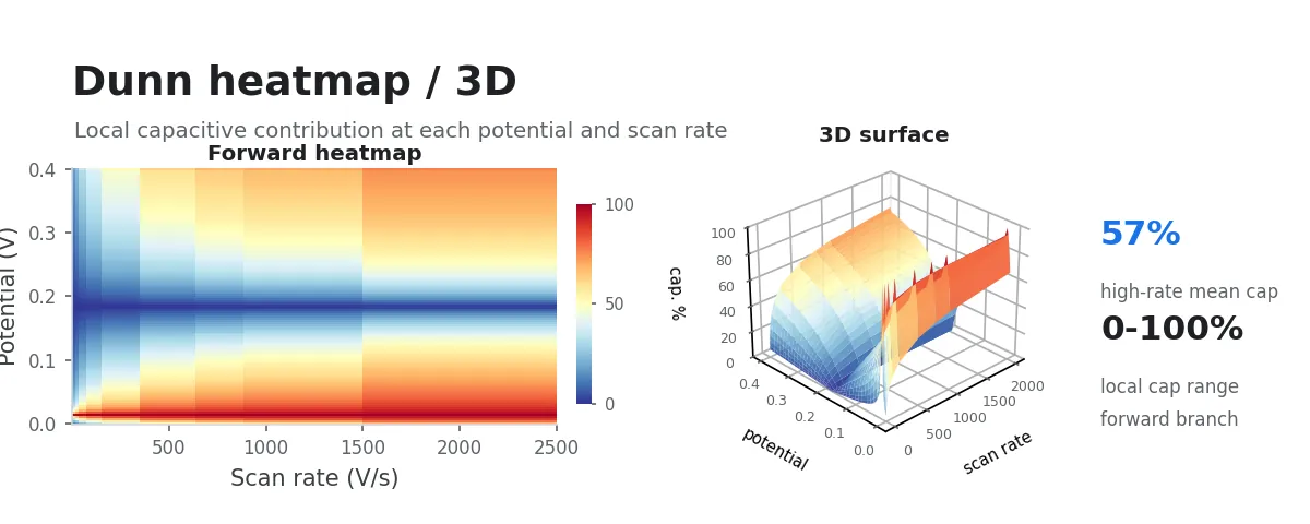
This workflow directly accepts a folder or multiple files of raw instrument-exported CV data. It uses Dunn’s method to compute the local capacitive contribution at every scan rate and every potential, then exports a 2D heatmap, fit-quality and residual diagnostics, result tables, an Origin project, and rotatable/zoomable 3D plots.

When To Use

The standard Dunn bar chart answers “what is the overall capacitive/diffusion contribution at each scan rate”. This workflow answers a more detailed question: “at a given scan rate, which potential regions are more capacitive-controlled and which are more diffusion-controlled”.

We recommend at least 3 distinct scan rates with a sufficiently wide shared potential window. The input may be a pseudocapacitive material, a mixed capacitive/diffusion-controlled system, or a purely capacitive baseline for validation.

Usage

Select a folder of raw CV data, or multi-select a group of raw CV files.
The workflow recognizes CV data automatically and computes forward/reverse potential-scan-rate contribution results in the shared potential window.
The result area shows a 2D heatmap, a text report, rotatable/zoomable contribution 3D plots, $R^2$ -potential fit-quality line plots, and residual heatmaps.
Click “生成 Origin 工程” to export an Origin project containing forward/reverse contribution heatmaps, $R^2$ line plots, residual heatmaps, and contribution 3D surfaces.

Method

Dunn’s method assumes that the current at each potential $E$ can be separated into capacitive and diffusion-controlled terms:

i(E, v) = k_1(E) \cdot v + k_2(E) \cdot v^{1/2}

Equivalently, the workflow fits the following relation at every potential:

\frac{i(E, v)}{v^{1/2}} = k_1(E) v^{1/2} + k_2(E)

After obtaining $k_1(E)$ and $k_2(E)$ , the local capacitive contribution at every scan rate $v$ and potential $E$ is calculated as:

C_{cap}(E, v) = \frac{|k_1(E)v|}{|k_1(E)v| + |k_2(E)v^{1/2}|} \times 100\%

The heatmap uses scan rate as the X axis, potential as the Y axis, and color as the local capacitive contribution percentage.

The fit-quality and residual results help identify which regions of the local contribution map deserve closer interpretation. $R^2$ describes the goodness of the Dunn linearized fit at each potential, computed in the linearized space of $i/\sqrt{v}$ versus $\sqrt{v}$ ; RMSE and NRMSE are reported in the original current space, representing the absolute current residual scale and the residual relative to the current magnitude, respectively. When a region has lower $R^2$ or higher NRMSE, interpret it together with the original CV curves.

Outputs

File	Description
`dunn_surface_heatmap.png`	2D heatmap image, with one subplot for forward scan and one for reverse scan
`dunn_surface_forward_matrix.csv`	Forward-scan local capacitive contribution table; rows are potentials and columns are scan rates
`dunn_surface_reverse_matrix.csv`	Reverse-scan local capacitive contribution table; rows are potentials and columns are scan rates
`dunn_surface_forward_long.csv`	Forward-scan result table for replotting in Origin or other graphing software
`dunn_surface_reverse_long.csv`	Reverse-scan result table for replotting in Origin or other graphing software
`dunn_surface_long.csv`	Combined forward/reverse result table
`dunn_surface_fit_quality.csv`	$R^2$ , RMSE, NRMSE, $k_1$ , and $k_2$ at every branch and potential
`dunn_surface_residuals.csv`	Measured current, fitted current, residual, and normalized residual at every branch, potential, and scan rate
`dunn_surface_fit_quality.png`	$R^2$ vs potential fit-quality line plot
`dunn_surface_residual_heatmap.png`	Forward/reverse normalized residual heatmap
`dunn_surface_report.md`	Text report
`dunn_surface_analysis.opju`	Origin project, generated when “生成 Origin 工程” is clicked and Origin is available

3D Interaction

The app result area displays the local capacitive contribution 3D plot inline; $R^2$ fit quality is shown as a potential line plot, while residuals are shown as heatmaps. You can rotate and zoom the contribution 3D surfaces and hover to inspect the capacitive contribution at the selected point; use the residual heatmap to quickly locate potential-scan-rate regions where the errors concentrate. Export the Origin project to view the contribution surface, $R^2$ line plot, and residual heatmap.

Interpretation

Colors closer to 100% indicate stronger capacitive/surface-controlled behavior at that potential and scan rate.
Colors closer to 0% indicate stronger diffusion-controlled behavior.
Reading along the potential axis at a fixed scan rate highlights potential regions with different storage mechanisms.
Reading along the scan-rate axis at a fixed potential shows whether the capacitive contribution increases with scan rate.

Notes

The heatmap and 3D plot show local contribution percentages, not the integrated contribution over the whole potential window. For systems involving phase transitions, precipitation reactions, strong irreversibility, or substantial noise, interpret the local contribution map together with the original CV curves and material mechanism.

References

Pu, X., Zhao, D., Fu, C., Chen, Z., Cao, S., Wang, C., and Cao, Y. (2021). Understanding and Calibration of Charge Storage Mechanism in Cyclic Voltammetry Curves. Angew. Chem. Int. Ed. 60, 21310-21318. DOI: 10.1002/anie.202104167.
Brezesinski, T., Wang, J., Tolbert, S.H., and Dunn, B. (2010). Ordered mesoporous alpha-MoO3 with iso-oriented nanocrystalline walls for thin-film pseudocapacitors. Nat. Mater. 9, 146-151. DOI: 10.1038/nmat2612.

CV/Dunn: Capacitive / Diffusion Contribution Ratio CV Data Extraction: Generic Format