CV/Randles-Sevcik: Diffusion Coefficient Calculation

Pro

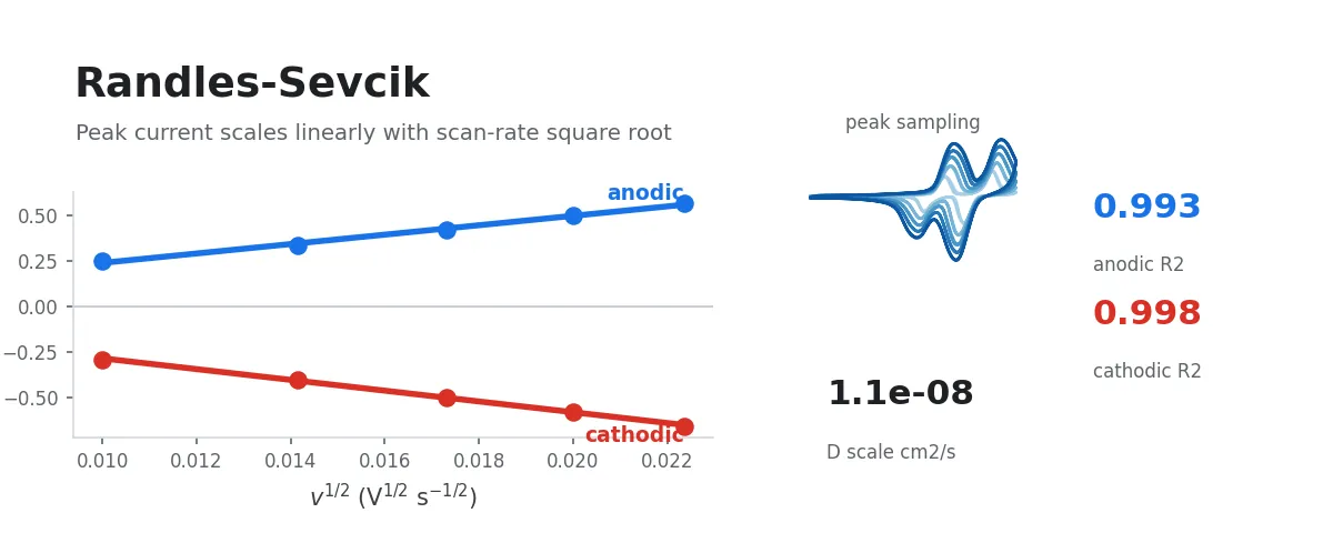
This workflow uses CV data recorded at different scan rates to automatically extract peak currents, then calculates the diffusion coefficient $D$ using the Randles-Sevcik equation.

Input Data

Select a folder containing instrument-exported raw CV data, or multi-select a group of raw CV data files.

The dataset should contain CV curves recorded at multiple scan rates.

Randles-Sevcik analysis depends on peak currents, so the input data should contain clear oxidation or reduction peaks. If the CV curves are close to purely capacitive rectangles and contain no clear peaks, this workflow exports candidate-peak and status information, but it does not use midpoint currents as substitutes for peak currents when calculating $D$ .

Procedure

Select input data: choose a folder containing CV data at different scan rates, or multi-select a group of data files.
Set the parameters:
- Electron-transfer number $n$
- Electrode area $A$ , in cm²
- Concentration $C$ , in mol/L
- Temperature $T$ , in K After editing the parameters, click “Apply parameters and calculate” to start or refresh the results.
The system automatically detects peaks, groups them across scan rates by scan branch and peak position, and fits $i_p$ versus $v^{1/2}$ for each valid peak group.
The workflow outputs fitting plots, a sample-point preview, summary tables, and intermediate data.
To create an Origin project, click “Generate Origin project”. Origin export is slow, so it does not run automatically when parameters are edited.

Scientific Principles

Reversible Randles-Sevcik equation:

i_p = 0.4463 n F A C \sqrt{\frac{n F v D}{R T}}

where:

Symbol	Meaning	Unit
$i_p$	Absolute peak current	A
$n$	Electron-transfer number	-
$F$	Faraday constant	C/mol
$A$	Electrode area	cm²
$C$	Bulk concentration	mol/cm³
$v$	Scan rate	V/s
$D$	Diffusion coefficient	cm²/s
$R$	Gas constant	J/(mol·K)
$T$	Temperature	K

The user-entered concentration is in mol/L; the workflow internally converts it to mol/cm³.

Writing the equation as $i_p = slope \cdot \sqrt{v} + intercept$ gives:

D = \left(\frac{|slope|}{0.4463 n F A C}\right)^2 \frac{R T}{n F}

The fit keeps an intercept so that background current or baseline offset can be inspected. Anodic peak currents are reported as positive values, while cathodic/reverse-scan peak currents are reported as negative values. The diffusion coefficient is calculated from the absolute value of the fitted slope.

Peak Selection Strategy

This workflow reuses the multi-peak processing strategy already validated in CV/Pseudocapacitance Analysis: b-Value Kinetic Analysis:

Candidate peaks are detected separately on the two one-directional scan segments of the last complete cycle in each scan-rate file.
Candidate peaks must pass prominence, endpoint-distance, and relative-current-height filters, reducing false positives from startup spikes or small fluctuations on capacitive plateaus.
Anodic and cathodic branches are grouped separately; visually symmetric oxidation and reduction peaks are not merged automatically.
A peak group must contain at least 3 distinct scan rates to report a valid $D$ .

Output

File	Content
`randles_sevcik_plot.png`	Grouped $i_p$ versus $v^{1/2}$ fitting plot. The x-axis is shown as `Scan Rate^{1/2} (V^{1/2} / s^{1/2})`; anodic and cathodic peak groups are drawn in the same plot, and the legend reports slope, $D$ , $R^2$ , and the number of scan rates used
`randles_sevcik_sample_points.png`	Sample-point preview showing all last-cycle CV curves in one overlay plot, with detected peak positions marked by `x`
`randles_sevcik_peaks.csv`	User-facing compact peak-point table, including group, branch, file name, scan rate, peak potential, signed peak current, raw current, point status, and source
`randles_sevcik_summary.csv`	One-row-per-group summary including the `slope_a_per_scan_rate_1_2` slope, intercept, $R^2$ , $D$ , parameters, and status
`randles_sevcik_fit_curves.csv`	Fitted-curve data
`randles_sevcik_analysis.opju`	Origin project, generated after clicking “Generate Origin project” when Origin is available; includes the Randles-Sevcik fit graph

Both randles_sevcik_plot.png and randles_sevcik_sample_points.png are displayed in the Workflow UI and saved to the output folder.

Scope

The first version is intended for reversible or approximately reversible Randles-Sevcik analysis. Irreversible and quasi-reversible systems use different equations and additional kinetic parameters, so this workflow should not be used as a direct replacement for those models.

Subsequent Analysis

CV/Pseudocapacitance Analysis: b-Value Kinetic Analysis: compare peak current against scan rate through a power-law relationship to distinguish diffusion-controlled, surface-controlled, and mixed-control behavior
CV/Cdl: Double-Layer Capacitance and Electrochemically Active Surface Area Analysis: calculate $C_{\text{dl}}$ from midpoint-current differences

References

Bard, A.J., and Faulkner, L.R. (2001). Electrochemical Methods: Fundamentals and Applications, 2nd ed. (John Wiley & Sons).
Randles, J.E.B. (1948). A cathode ray polarograph. Part II. The current-voltage curves. Trans. Faraday Soc. 44, 327-338. DOI: 10.1039/TF9484400327.
Sevcik, A. (1948). Oscillographic polarography with periodical triangular voltage. Collect. Czechoslov. Chem. Commun. 13, 349-377. DOI: 10.1135/cccc19480349.
Nicholson, R.S., and Shain, I. (1964). Theory of stationary electrode polarography. Single scan and cyclic methods applied to reversible, irreversible, and kinetic systems. Anal. Chem. 36, 706-723. DOI: 10.1021/ac60210a007.

CV/Pseudocapacitance Analysis: b-Value Kinetic Analysis CV/Cdl: Double-Layer Capacitance and Electrochemically Active Surface Area Analysis