EIS Blank Subtraction

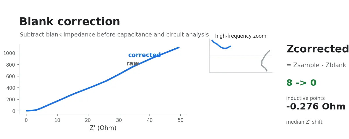
In low-impedance systems or high-frequency EIS measurements, cables, fixtures, and connectors can contribute measurable impedance. This workflow subtracts the complex impedance of a blank circuit measured under the same conditions from the experimental data, producing corrected EIS data that better represent the device under test.

It is useful before comparing ohmic resistance, interpreting high-frequency response, running DRT analysis, or performing equivalent-circuit fitting. The workflow does not assign a material mechanism; it only removes the part of the measured impedance that can be represented by the blank measurement.

Why Blank Subtraction Is Needed

An EIS instrument measures the impedance of the entire test loop, not only the sample. For low-impedance devices, the resistance introduced by cables and fixtures can be non-negligible. At high frequency, cable inductance can also shift the imaginary component of the response.

The measured impedance can be approximated as:

If the blank circuit and the sample are measured with the same cables, fixtures, and test parameters:

The key point is that the blank measurement directly characterizes the contribution of the test loop; the workflow does not require fitting a specific circuit element.

When to Use It

This workflow is recommended when:

• The sample has very low ohmic impedance, for example in the 10-100 mΩ range
• The EIS measurement uses a high maximum frequency, for example above 100 kHz
• The high-frequency Nyquist response is affected by cables or fixtures
• You plan to run EIS/DRT Analysis: Mapping Frequency-Domain Impedance to a Distribution of Relaxation Times or equivalent-circuit fitting
• You need to compare impedance differences across samples, batches, or fixture conditions

For conventional data with larger impedance and a moderate frequency range, the curves may change only slightly after blank subtraction. This is expected.

Input Data

You can directly select a folder containing instrument-exported raw EIS data, or select multiple experimental data files. The workflow automatically recognizes common text, CSV, Excel, EC-Lab .mpr, Gamry .dta, VersaStudio .par, and similar formats, then converts them into the internal standardized EIS table.

Select the blank from the original instrument-exported EIS data as well.

How to Measure the Blank

The blank should represent only the response of the test leads, fixtures, and connectors as much as possible. A common approach is to remove the device under test, directly short the two electrode clips that would normally hold the device, and run one EIS measurement using exactly the same parameters as the sample measurement.

Keep the following conditions consistent:

• Frequency range and frequency points
• AC perturbation amplitude
• Rest time and measurement mode
• Cable, fixture, connector, and physical placement conditions

The closer the frequency lists are, the more reliable the subtraction will be. If the sample and blank use different frequency points, the workflow can only subtract points that can be matched.

Calculation Logic

For each sample, the workflow finds the nearest frequency point in the blank data. The default relative frequency tolerance is 2%. When a frequency point is matched, the real and imaginary components are subtracted separately:

It then recalculates:

• z_mod_ohm: impedance magnitude after subtraction
• phase_deg: phase angle after subtraction
• c_f: point-wise capacitance estimate when the corrected imaginary part is capacitive

Rows without a matched blank frequency point are kept, but they are marked as compensated = False and their corrected values are left empty.

Procedure

1. Select the experimental EIS data, either as a raw data folder or as multiple experimental data files.
2. Select the blank EIS data file, such as an instrument-exported raw file or a standardized blank_eis.csv.
3. The workflow automatically excludes the blank file itself and older *_corrected_eis.csv outputs, processing only recognizable experimental EIS data.
4. After processing, inspect the corrected CSV files, comparison plots, and diagnostic report in the output folder.

Output

The workflow creates a base_correction_output folder under the input directory.

Each sample produces:

• {sample}_corrected_eis.csv: standardized EIS data after blank subtraction
• {sample}_nyquist_comparison.png: Nyquist comparison before and after subtraction, with the highest-frequency 20% region enlarged on the right

Summary files include:

• corrected_summary.csv: input file, blank file, output file, and matched-point count for each sample
• correction_diagnostics.csv: frequency matching ratio and diagnostic information
• correction_diagnostics.md: a short human-readable diagnostic report

After clicking “Confirm generation”, the workflow also exports:

• base_correction_nyquist.opju: an Origin project containing Nyquist comparisons before and after subtraction

Corrected CSV Columns

How to Interpret the Results

Start with {sample}_nyquist_comparison.png:

• Gray Raw points show the original EIS data
• Blue Corrected points show the data after blank subtraction
• The right panel enlarges the highest-frequency 20% of points to make high-frequency changes easier to inspect

Then review correction_diagnostics.md or correction_diagnostics.csv:

• The closer n_compensated / n_points is to 100%, the more consistent the sample and blank frequency lists are
• If the frequency matching ratio is below 90%, check whether the blank was measured with the same test parameters
• If no points are matched, the blank file is usually wrong or the sample and blank frequency lists differ too much

Subsequent Analysis

The *_corrected_eis.csv files keep the standard z_real_ohm and z_imag_ohm columns, so they can be used directly by:

• EIS Plotting: Nyquist and Bode Visualization: re-plot Nyquist and Bode diagrams
• EIS/DRT Analysis: Mapping Frequency-Domain Impedance to a Distribution of Relaxation Times: run DRT analysis on the corrected impedance
• Equivalent-circuit fitting: reduce the influence of parasitic test-loop response on high-frequency fitting

Notes

• Blank subtraction cannot fix unstable measurements, poor contact, or sample drift.
• The blank should use the same cable and fixture configuration as the sample as much as possible; otherwise the subtraction can introduce new bias.
• If the corrected high-frequency real part becomes clearly unreasonable or negative, check the blank measurement and confirm that the sample and blank used the same test parameters.