EIS/DRT Analysis: Mapping Frequency-Domain Impedance to a Distribution of Relaxation Times

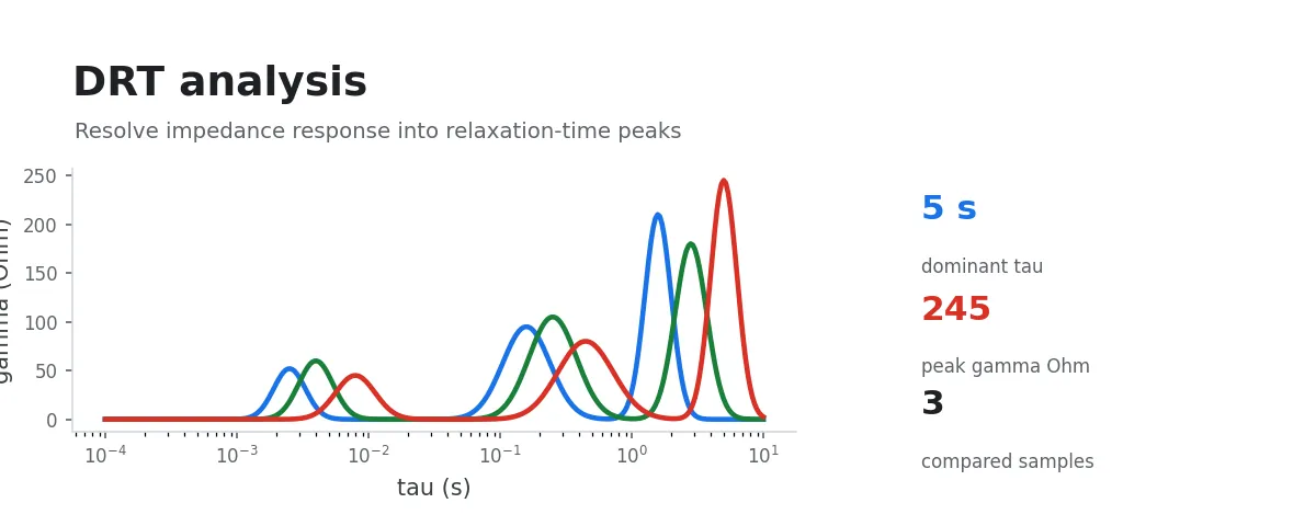
If you have already reviewed the Nyquist and Bode plots but want to understand which kinetic process is dominating the response, this workflow is designed for exactly that purpose.

It performs DRT (Distribution of Relaxation Times) analysis on EIS data, mapping frequency-domain impedance information onto a time-constant distribution. This makes it much easier to distinguish different processes visually (e.g., interfacial charge transfer, diffusion-related processes, etc.).

Input Data

Select a folder containing instrument-exported raw EIS data, or multi-select a group of raw EIS data files.

Procedure

You have two options:

1. Select a directory (batch-process all recognizable EIS data in it)
2. Or multi-select a group of files (useful when analyzing only part of an experiment)

The program automatically creates a drt_output directory and outputs results for each sample separately.

Analysis and Fitting Results

Each sample produces the following data files:

• fit_data.csv: experimental impedance, DRT-reconstructed impedance, and residuals
• drt_data.csv: $\tau$ and $\gamma(\tau)$ distribution
• summary.json: regularization parameters and solver summary (e.g., lambda_value, epsilon)

Along with the following visualization plots:

• nyquist_fit.png: experimental vs. DRT-fitted Nyquist comparison
• drt_tau.png: $\gamma$–$\tau$ distribution plot (log-scale x-axis)
• residuals.png: real/imaginary residual plot
• *_drt_plots.opju: Origin project (containing Nyquist, DRT, and residual plots)

Principle (Brief)

DRT represents impedance as a superposition of processes with different time constants. The core idea can be written as:

Where:

• The peak positions of $\gamma(\tau)$ reflect the characteristic time scales of different processes
• The peak area and height relate to the contribution strength of each process

This approach makes it significantly easier to resolve overlapping mechanisms compared to interpreting Nyquist semicircles alone.

FAQ

• Why are there no results for some samples? The most common reason is missing input columns or invalid values in the data. The program skips these samples and reports the specific error.

Practical Tips

If this is your first time running DRT, it is a good idea to use EIS Plotting: Nyquist and Bode Visualization first to verify that the curves are smooth and free of obvious outliers. Doing so before entering this step typically yields more stable and more interpretable results.